In 1881, the astronomer Simon Newcomb noticed that the first pages of logarithm tables wore out faster than the last ones. In 1938, Frank Benford, a physicist at General Electric, confirmed the same pattern with more than twenty thousand numbers: in many real-world datasets, about three-tenths of numbers begin with 1, while less than 5% begin with 9. The pattern was later used in auditing and election checks, but it can only point to data that deserve a second look. On its own, it cannot prove fabrication.
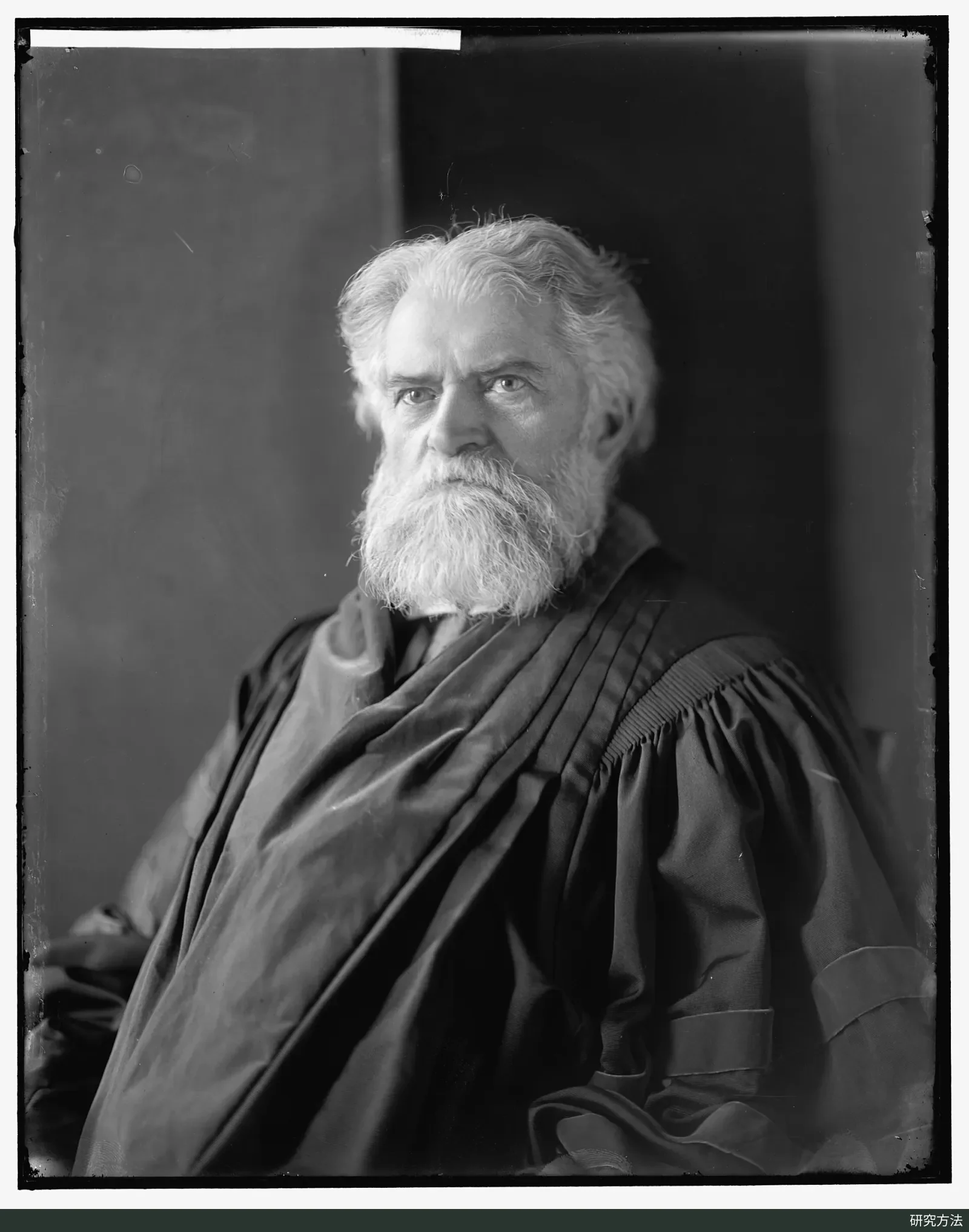
Portrait of Simon Newcomb, taken around 1905 to 1909. Photograph: Harris & Ewing; source: Library of Congress collection (via Wikimedia Commons); license: public domain.

What Newcomb and Benford Observed
Simon Newcomb was an American astronomer and mathematician. In 1881, he published a short note of just two pages in volume 4 of the American Journal of Mathematics, titled “Note on the Frequency of Use of the Different Digits in Natural Numbers.” The note begins with an observation: anyone who uses logarithm tables often will notice that the first pages wear out much faster than the last ones. Before calculators existed, multiplication and division required looking up logarithms in tables. The numbers in those tables were listed in order of size, so numbers beginning with 1 came first. Because the first pages wore out faster, more of the numbers people looked up must have begun with 1.
From this, Newcomb inferred that the first significant digit is 1 more often than any other digit, and that the frequencies decrease steadily from 1 to 9. He argued that numbers found in nature can be regarded as ratios of quantities. After repeated division, the fractional parts of their logarithms (the mantissas) tend toward a uniform distribution. He therefore concluded that “all mantissas of logarithms are equally probable.” He also used this idea to calculate probabilities for the first two digits. According to his table, the second digit is already close to uniform, with 0 at about 11.97% and 9 at about 8.50%. By the third digit, every digit has almost the same probability.
More than half a century later, Frank Benford, a physicist at the General Electric research laboratory, carried out a large-scale count. His paper “The Law of Anomalous Numbers” was read before the American Philosophical Society on April 22, 1937, and published in March 1938 in volume 78 of the Proceedings of the American Philosophical Society. Benford collected 20 groups of data containing a total of 20,229 observations. His sources included river areas, U.S. populations, physical constants, numbers printed in newspapers, specific heats, molecular weights, American League baseball statistics for 1936, street addresses from American Men of Science, and death rates. Averaged across the 20 groups, 30.6% of the numbers began with 1, and only 4.7% began with 9.
Benford also found that a single group of data did not necessarily fit the pattern. In the atomic-weight group, 47.2% of the numbers began with 1, and in the physical-constant group, 41.3% did. Unrelated numbers mixed together, such as the assorted numbers taken from newspapers, actually fit the logarithmic distribution better. He called these “anomalous numbers”: individual numbers that have no connection with one another, but that follow the same distribution when they appear in large batches. The pattern was later named after him.
Explanations Based on Scale Invariance and Mixed Distributions
Benford's law is usually written as follows: the probability that the first digit is d is P(d) = log₁₀(1 + 1/d), where d ranges from 1 to 9. Working out the values gives about 30.1% for 1, about 17.6% for 2, and about 12.5% for 3, falling steadily to about 4.6% for 9. This is equivalent to Newcomb's statement: if you write a number in scientific notation and take its base-10 logarithm, the fractional part is uniformly distributed between 0 and 1. Numbers whose first digit is 1 have fractional parts between 0 and log₁₀2 (about 0.301). This interval is the longest one, so 1 appears most often.
A quantity that grows by a fixed percentage makes this easier to picture. Suppose a city's population grows by 10% each year. Growing from 1 million to 2 million takes about 7.3 years, and the population figure begins with 1 for that entire period. Growing from 9 million to 10 million takes only about 1.1 years, so the stage where the figure begins with 9 passes quickly. If you check data like this at a random moment, you are naturally more likely to see 1 as the first digit.
In 1961, Roger Pinkham proved in The Annals of Mathematical Statistics that if a first-digit distribution does not change with the unit of measurement, meaning the proportions stay the same whether values are recorded in dollars or euros, meters or feet, then that distribution can only be log₁₀(1 + 1/d). A distribution in which “all nine digits are equally likely” does not survive a change of units: if every number is multiplied by 2, all the numbers that previously began with 5 through 9 will begin with 1.
Scale invariance explains “what shape such a law would have to take, if one exists,” but it does not explain why real data behave this way. In 1995, Theodore Hill offered a statistical explanation in Statistical Science. Suppose many different distributions are first chosen at random in a way that favors no particular scale, a sample is then drawn from each distribution, and all the samples are pooled. The first-digit frequencies will converge to the Benford distribution. This result does not require each individual distribution to obey Benford's law. That matches Benford's own observation: single tables often fit poorly, while data combined from many sources fit better.
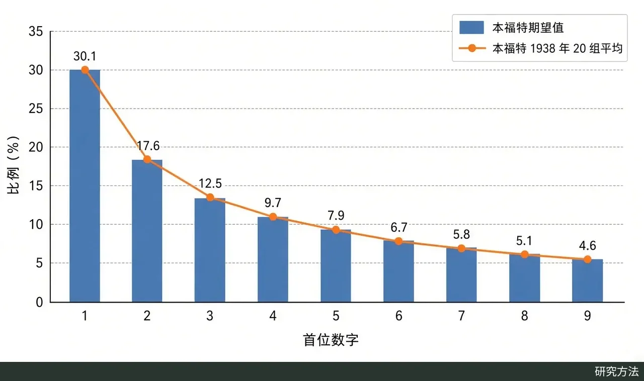
Expected proportions of first digits (bars, computed from log₁₀(1 + 1/d)) and the averages of the 20 data groups in Table I of Benford's 1938 paper (dots). Data source: Benford (1938); plotted for this article with Python code.
Uses in Financial and Election Data
The idea of using this pattern as a checking tool emerged in the 1970s. According to Hill's 1995 review, the economist Hal Varian suggested in 1972 that how closely data fit the logarithmic distribution could be used to test whether a model's output was reasonable. The accounting scholar Mark Nigrini later applied the pattern systematically to tax data. His 1996 study in The Journal of the American Taxation Association distinguished between two kinds of tax evasion. “Unplanned evasion” involves making up figures on the spot while filing a return, while “planned evasion” involves hiding the audit trail in advance. His premise was that honestly reported figures and carefully arranged figures should both follow the Benford distribution, while figures made up on the spot would leave deviations. After analyzing the IRS's individual tax sample files, he concluded that low-income taxpayers made up figures on the spot to a greater extent than high-income taxpayers.
This kind of test soon entered professional practice. In his 1995 paper, Hill cited a Wall Street Journal report from July of that year: the Brooklyn District Attorney's office in New York had used Nigrini's Benford goodness-of-fit test to uncover and prosecute a fraud ring involving 7 New York companies. A 2004 guide for auditors by Durtschi et al. argued that most accounting data are suitable for this check, because accounts receivable, accounts payable, and most revenue and expense accounts are produced by calculations such as “quantity times unit price.” The authors also recommended analyzing entire accounts rather than samples, because the more data there are, the more reliable the results.
Election data are another area of use, and a more controversial one. Starting in 2006, the political scientist Walter Mebane proposed testing the second digits of precinct vote counts, an approach often called the “2BL test.” At the time, he noted that the test cannot detect every type of fraud, and that vote counts with no fraud can also produce significant results. He advised against examining first digits, partly because of an example given by Henry Brady in 2005. If two candidates are evenly matched and precincts contain between 100 and 1000 voters, the most common first digit of each candidate's vote count is 4, 5, or 6, not 1 or 2.
In 2011, Joseph Deckert, Mikhail Myagkov, and Peter Ordeshook published an article in Political Analysis that tested simulated fair and fraudulent elections. They also tested real elections that other investigations had either confirmed as fraudulent or found to be essentially free of fraud. Their conclusion was that there was no visible link between whether the data fit Benford's law and whether an election was fraudulent. The test's “success rate” was roughly equal to that of a coin toss. In a commentary in the same issue, Mebane criticized their simulation design and the level at which they aggregated the data. Even so, he agreed that a second-digit mean significantly different from 4.187 is not, by itself, evidence of fraud. Whether such tests are useful remains an open question, and expected patterns need to be set according to the characteristics of real elections.
Unsuitable Data and the Limits of the Test
The Benford distribution suits data that span several orders of magnitude and are produced by a combination of many factors. Durtschi et al. listed several kinds of data that usually do not fit it. The first kind is assigned numbers, such as check numbers, invoice numbers, and postal codes. These numbers are issued in sequence or according to rules, so their first digits are closer to a uniform distribution. The second kind is numbers shaped by human choices, such as prices set at psychological price points like $1.99, or preset round amounts such as ATM withdrawals. The third kind is truncated data with built-in minimums or maximums, such as an asset list that records only items above a materiality threshold. Brady's precinct example above also falls into this category: precinct size limits vote counts to a range narrower than one order of magnitude, so the first digits naturally cluster around the middle values. Durtschi et al. also gave a rough rule of thumb: if a dataset's mean is greater than its median and the data are positively skewed, the data are more likely to fit the Benford distribution. The figure below uses simulated data to compare three cases.
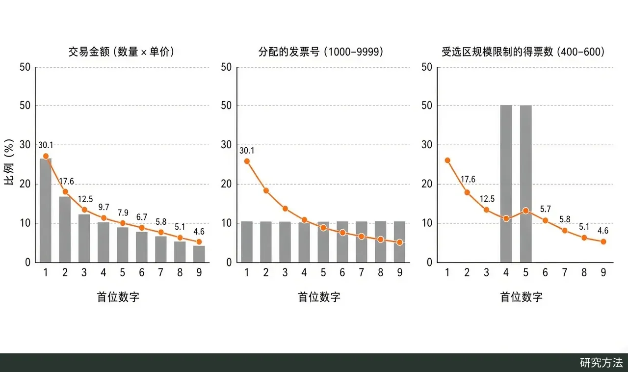
First-digit distributions of three simulated datasets, with the orange line showing the expected Benford proportions. Left: transaction amounts calculated by multiplying quantity by unit price; middle: invoice numbers assigned uniformly from 1000–9999; right: vote counts limited by precinct size to 400–600. Simulated data, plotted for this article with Python code.
Even when the data are the right type, a deviation from the Benford distribution cannot prove fabrication on its own. Deviations can come from normal business rules, rounding, recording thresholds, and pricing habits. Conversely, data that fit the distribution are not necessarily clean. Nigrini's own study assumes that carefully arranged “planned evasion” figures will still follow the Benford distribution. Durtschi et al. also noted that digit analysis cannot detect frauds that never enter the books at all, such as theft, kickbacks, and bid-rigging. When setting “how large a deviation counts as suspicious,” analysts must also weigh the costs of false positives against those of false negatives. The election debate shows that there is not even an agreed model of “what fraud-free vote counts should look like.”
The Benford test is therefore better used as a screening tool. First, decide whether this kind of data should follow the distribution. Next, see which digits, accounts, or precincts the deviations are concentrated in. Finally, confirm any problem with independent evidence, such as checking source documents or conducting on-site investigations. As Mebane wrote in his 2006 paper, perhaps one should not expect too much from a test that can work only with the vote counts themselves.
The two statistical figures in this article can be reproduced with the Python code below, which requires NumPy and Matplotlib. Benford's 1938 averages are taken from the last row of Table I in his paper.
import numpy as np
import matplotlib.pyplot as plt

plt.rcParams["font.sans-serif"] = ["Noto Sans CJK SC", "Microsoft YaHei", "SimHei", "DejaVu Sans"]
plt.rcParams["axes.unicode_minus"] = False

digits = np.arange(1, 10)
benford = np.log10(1 + 1 / digits)
# Average row of Table I in Benford (1938), in percent
benford_1938 = np.array([30.6, 18.5, 12.4, 9.4, 8.0, 6.4, 5.1, 4.9, 4.7])


def first_digit(x):
    x = np.asarray(x, dtype=float)
    x = x[x > 0]
    # Small offset guards against log10(1000) evaluating to 2.999...
    scaled = x / 10 ** np.floor(np.log10(x) + 1e-12)
    return np.clip(scaled.astype(int), 1, 9)


def digit_share(x):
    d = first_digit(x)
    return np.array([(d == k).mean() for k in digits])


# Figure 1: expected shares vs. Benford's 1938 average
fig, ax = plt.subplots(figsize=(7, 4))
bars = ax.bar(digits, benford * 100, color="#4C72B0", label="本福特期望值")
ax.bar_label(bars, fmt="%.1f")
ax.plot(digits, benford_1938, "o-", color="#DD8452", label="本福特 1938 年 20 组平均")
ax.set_xticks(digits)
ax.set_xlabel("首位数字")
ax.set_ylabel("比例(%)")
ax.legend()
fig.tight_layout()
fig.savefig("benford_expected.png", dpi=200)

# Figure 2: three simulated datasets
rng = np.random.default_rng(1938)
n = 10_000
amounts = rng.integers(1, 51, n) * rng.lognormal(mean=3, sigma=1.2, size=n)
invoices = rng.integers(1000, 10000, n)
votes = np.round(1000 * rng.uniform(0.40, 0.60, n))
panels = [
    ("交易金额(数量×单价)", amounts),
    ("分配的发票号(1000–9999)", invoices),
    ("受选区规模限制的得票数(400–600)", votes),
]

fig, axes = plt.subplots(1, 3, figsize=(12, 3.8), sharey=True)
for ax, (title, data) in zip(axes, panels):
    ax.bar(digits, digit_share(data) * 100, color="#8C8C8C")
    ax.plot(digits, benford * 100, "o-", color="#DD8452")
    ax.set_title(title)
    ax.set_xticks(digits)
    ax.set_xlabel("首位数字")
axes[0].set_ylabel("比例(%)")
fig.tight_layout()
fig.savefig("benford_compare.png", dpi=200)
References
-
Newcomb, S. (1881). Note on the Frequency of Use of the Different Digits in Natural Numbers. American Journal of Mathematics, 4(1), 39–40. doi:10.2307/2369148
-
Benford, F. (1938). The Law of Anomalous Numbers. Proceedings of the American Philosophical Society, 78(4), 551–572. JSTOR 984802
-
Pinkham, R. S. (1961). On the Distribution of First Significant Digits. The Annals of Mathematical Statistics, 32(4), 1223–1230. doi:10.1214/aoms/1177704862
-
Hill, T. P. (1995). A Statistical Derivation of the Significant-Digit Law. Statistical Science, 10(4), 354–363. doi:10.1214/ss/1177009869
-
Nigrini, M. J. (1996). A Taxpayer Compliance Application of Benford's Law. The Journal of the American Taxation Association, 18(1), 72–91. doi:10.2308/jata-6148128
-
Durtschi, C., Hillison, W., & Pacini, C. (2004). The Effective Use of Benford's Law to Assist in Detecting Fraud in Accounting Data. Journal of Forensic Accounting, 5(1), 17–34. USF Digital Commons
-
Deckert, J., Myagkov, M., & Ordeshook, P. C. (2011). Benford's Law and the Detection of Election Fraud. Political Analysis, 19(3), 245–268. doi:10.1093/pan/mpr014
-
Mebane, W. R., Jr. (2011). Comment on "Benford's Law and the Detection of Election Fraud". Political Analysis, 19(3), 269–272. doi:10.1093/pan/mpr024
-
Research Methods · Rituals can be imitated; understanding cannot be faked
-
Compiled and published by Scholay Academic One-Stop Platform. If any content infringes your rights, please contact us and it will be taken down.
-
Also published on EnterScholar, a community for scholars in the age of AI